HPC-T-Annotator

Step-by-step example of a typical usecase
Immagine that you want to run the BLASTX software on a transcriptome file input.fa against the NR database. You have an HPC cluster at your disposal. And after the alignment is done, you want to interpret the results showing some meaningful information about your transcriptome.
Step 1: Configure the Workload Manager Settings
Assume you have to run the BLASTX software on a transcriptome file input.fa against the NR database.
Let
- /home/user/assembly/input.fa be the transcriptome file's absolute path and
- /home/user/DATABASES/NR be the database's absolute path.
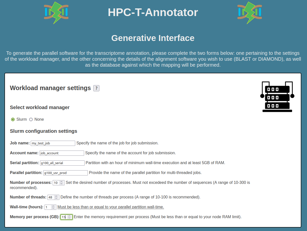
Suppose also that you have an HPC cluster, with the SLURM workload manager, at your disposal. Both the transcriptome file and the database (and the executable binary as well) are already available on the cluster. You can run HPC-T-Annotator on your cluster by generating all the necessary files through our interface, filling out the form as follows.
Now, you must fill the second part of the form with the following alignment software settings:
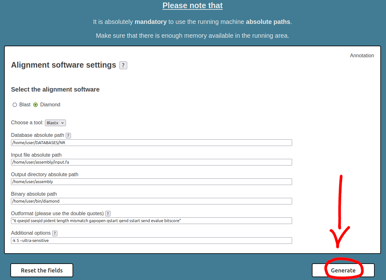
The images above show the filled HPC-T-Annotator interface. In this context, we have assumed that:
- Job name: is "my_test_job".
- Account name: is "job_account".
- Serial partition: is "g100_all_serial".
- Parallel partition: is "g100_usr_prod".
- Number of Processes: is 10.
- Number of Threads: is 48.
- Wall time (hours): is 1.
- Memory per process (GB): is 15.
and the following software settings:
- Alignment Software: is Diamond.
- Tool: is BLASTX.
- Database: is /home/user/DATABASES/NR.
- Input file: is /home/user/assembly/input.fa.
- Outdir: is /home/user/assembly.
- Binary: is /home/user/bin/diamond.
- Outformat: is "6 qseqid sseqid pident length mismatch gapopen qstart qend sstart send evalue bitscore".
- Additional options: are -k 5 --ultra-sensitive.
Now, all we have to do is click on the "Generate" button and the interface automatically generates the software package in TAR format.
Step 2: Upload and Run the Software Package to the HPC Cluster
You can now upload the package to your HPC cluster using the scp Unix command as follows:
Where cluster_domain is the domain name of the HPC cluster, /path/to/your/work/directory is the path where the software package is uploaded, and user is the username of your account on the HPC cluster.
Now, you have to extract the software package using the tar Unix command as follows:
After that, you can run the start.sh script on the HPC cluster using the following command:
After the computation process has ended (check the general.log file for the status), the final result will be in the /home/user/assembly/final_blast.tsv file.
Step 3: Results Analysis
Once the entire computation process has ended (check the general.log file for the status), you can download the /home/user/assembly/final_blast.tsv file using the scp Unix command as follows:
Where cluster_domain is the domain name of the HPC cluster, /path/to/your/work/directory is the path where the software package is uploaded, and user is the username of your account on the HPC cluster.
Now, you have to choose how to use the Jupyter notebooks to visualize the results. You can use these three options:
- - Google Colab: you can use the Jupyter notebooks in Google Colab. Remember that you have to load the TSV results file into your Google Colab environment before.
- - Docker: you can open the Jupyter notebooks in this Docker environment. Please follow the instructions in the README file or in this YouTube video to correctly configure and run the Docker environment. In this case, remember to put the TSV results file in the /path/to/your/work/results directory that you have linked to the Docker container.
- - Customized: you can open the Jupyter notebooks in a customized environment. For example, you can use the Anaconda Jupyter/Jupyter Lab environment to perform the entire analysis.
Results Analysis with Google Colab
Let's now analyze the results using the Google Colab option.
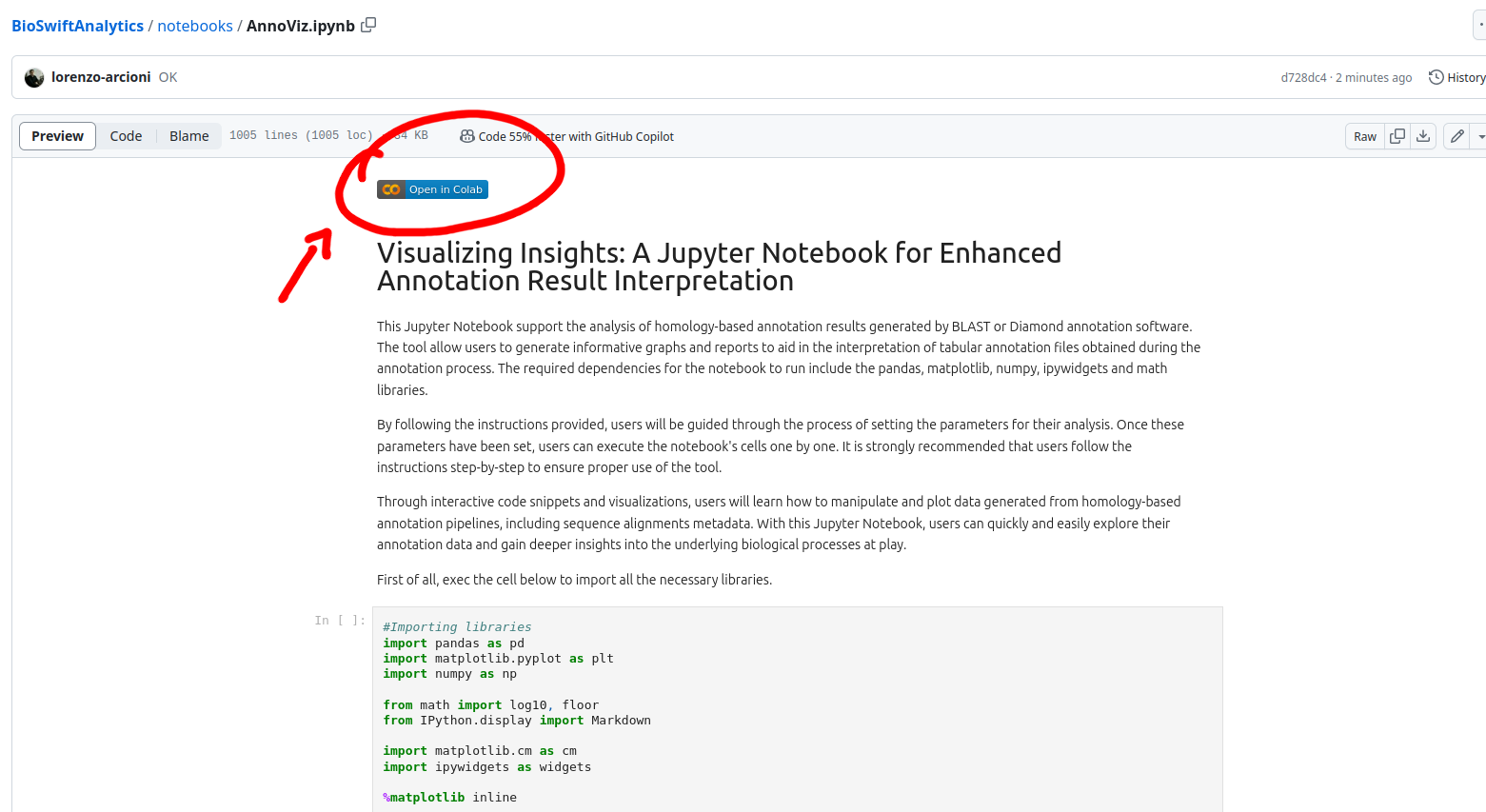
First, open the GitHub repository of BioSwiftAnalytics and select a notebook from the directory notebooks and click on the Colab button.
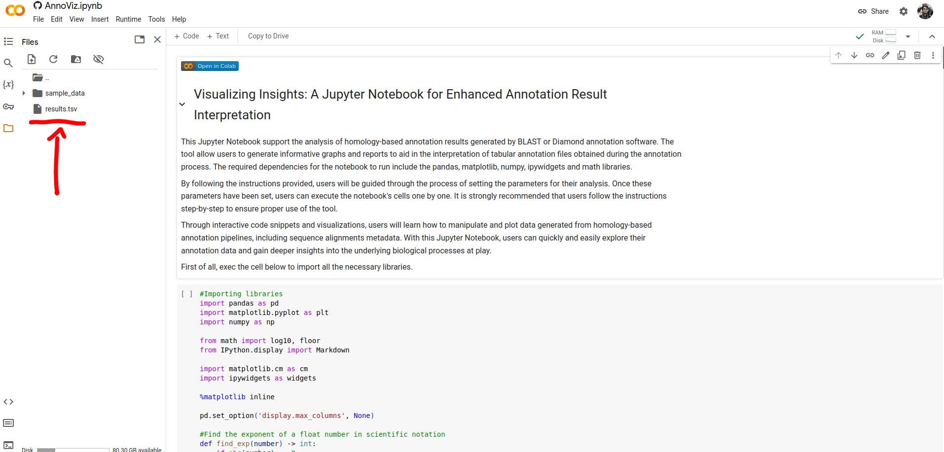
Now, you can load the TSV results file into your Jupyter environment dragging and dropping it.
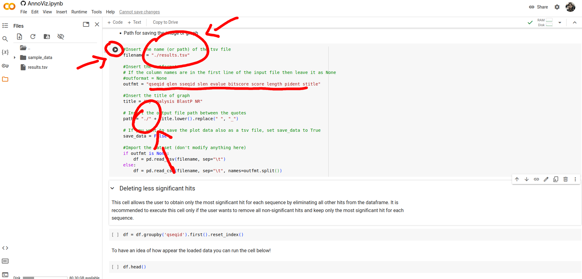
Now, you have to fill, with your data, the notebook's cell parameters. In particular, you need to specify the path of the TSV results file, the execution outformat, and the output directory. And next, you can click on the Run button.
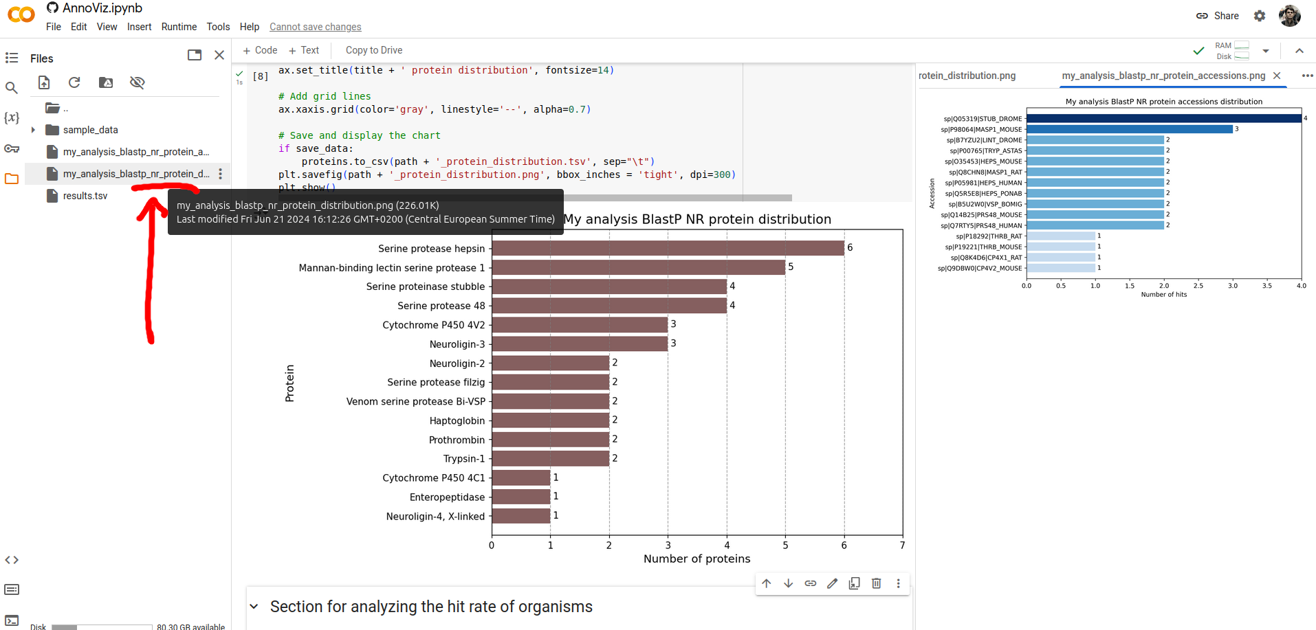
After executing all notebook's cells,
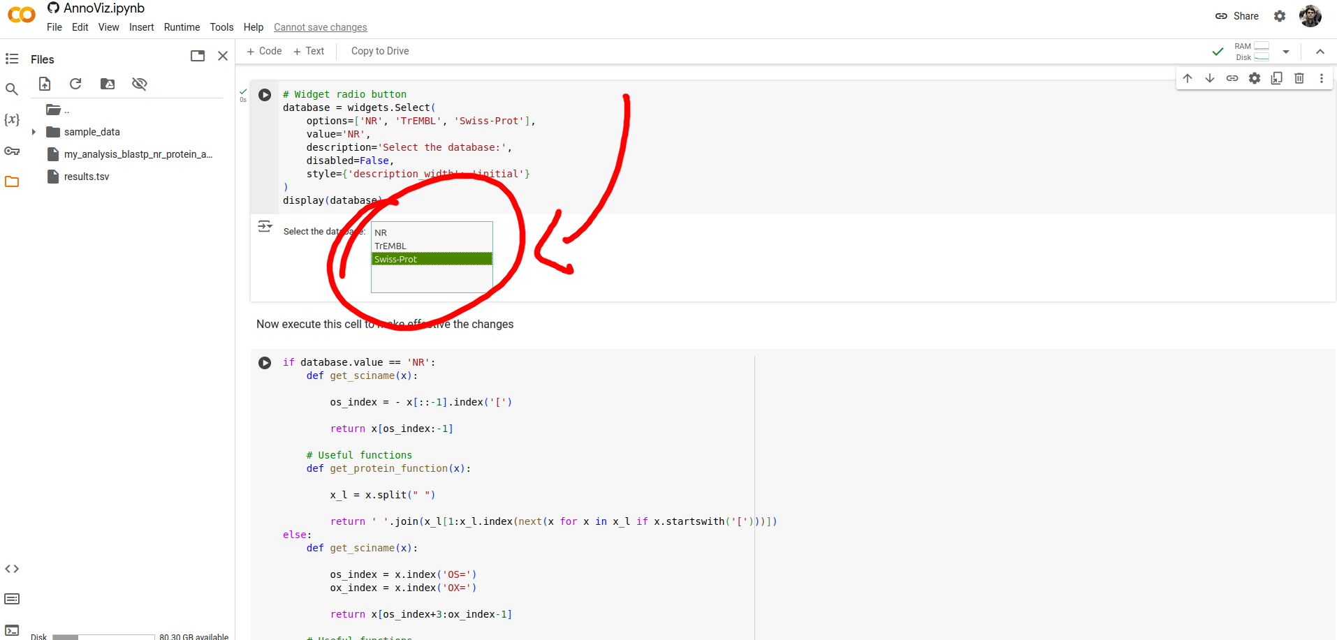
you can download the results from the Colab cloud space directory.
